0%

kaggle

Python

list

  • 遍历list
list = ["01", "02", "03", "04"]
# 1
for num in list:
print(num)

# 2
for i in range(len(list)):
print(list[i])

# 3
for num in iter(list):
print(num)

# 4
for obj in enumerate(list):
print(obj)
for index, value in enumerate(list):
print("index =", index, "value =", value)
  • 比较list元素, [False, True, True, False]
# 使用列表推导式
print([x > 2 for x in a])

# 使用 map 函数
print(list(map(lambda x: x > 2, a)))

dict

def multi_word_search(doc_list, keywords):
"""
Takes list of documents (each document is a string) and a list of keywords.
Returns a dictionary where each key is a keyword, and the value is a list of indices
(from doc_list) of the documents containing that keyword

>>> doc_list = ["The Learn Python Challenge Casino.", "They bought a car and a casino", "Casinoville"]
>>> keywords = ['casino', 'they']
>>> multi_word_search(doc_list, keywords)
{'casino': [0, 1], 'they': [1]}
"""
indices = {}
for x in keywords:
indices[x] = []
for i, doc in enumerate(doc_list):
tokens = doc.split()
normalized = [token.rstrip('.,').lower() for token in tokens]
for x in keywords:
if x.lower() in normalized:
indices[x].append(i)
return indices
  • 判断key是否在dict中
dict = {'name': '','age': '','sex': ''}
# 1
print(dict.has_key('name'))
# 2
print('name' in dict.keys())
# 3
print('name' in dict) # 结果返回True

Pandas

Creating, Reading and Writing

import pandas as pd

Creating data:There are two core objects in pandas: the DataFrame and the Series.

DataFrame
pd.DataFrame({'Yes': [50, 21], 'No': [131, 2]})
Yes No
0 50 131
1 21 2
pd.DataFrame({'Bob': ['I liked it.', 'It was awful.'], 'Sue': ['Pretty good.', 'Bland.']})
Bob Sue
0 I liked it. Pretty good.
1 It was awful. Bland.
pd.DataFrame({'Bob': ['I liked it.', 'It was awful.'], 
'Sue': ['Pretty good.', 'Bland.']},
index=['Product A', 'Product B'])
Bob Sue
Product A I liked it. Pretty good.
Product B It was awful. Bland.
Series
pd.Series([1, 2, 3, 4, 5])
0    1
1 2
2 3
3 4
4 5
dtype: int64
pd.Series([30, 35, 40], index=['2015 Sales', '2016 Sales', '2017 Sales'], name='Product A')
2015 Sales    30
2016 Sales 35
2017 Sales 40
Name: Product A, dtype: int64

Indexing, Selecting & Assigning

reviews
country description designation points price province region_1 region_2 taster_name taster_twitter_handle title variety winery
0 Italy Aromas include tropical fruit, broom, brimston… Vulkà Bianco 87 NaN Sicily & Sardinia Etna NaN Kerin O’Keefe @kerinokeefe Nicosia 2013 Vulkà Bianco (Etna) White Blend Nicosia
1 Portugal This is ripe and fruity, a wine that is smooth… Avidagos 87 15.0 Douro NaN NaN Roger Voss @vossroger Quinta dos Avidagos 2011 Avidagos Red (Douro) Portuguese Red Quinta dos Avidagos
129969 France A dry style of Pinot Gris, this is crisp with … NaN 90 32.0 Alsace Alsace NaN Roger Voss @vossroger Domaine Marcel Deiss 2012 Pinot Gris (Alsace) Pinot Gris Domaine Marcel Deiss
129970 France Big, rich and off-dry, this is powered by inte… Lieu-dit Harth Cuvée Caroline 90 21.0 Alsace Alsace NaN Roger Voss @vossroger Domaine Schoffit 2012 Lieu-dit Harth Cuvée Car… Gewürztraminer Domaine Schoffit
  • 查看某列
reviews.country # reviews['country']
0            Italy
1 Portugal
...
129969 France
129970 France
Name: country, Length: 129971, dtype: object
  • 查看某列的某一行
reviews['country'][0]
'Italy'
iloc

loc和iloc都是行第一,列第二, iloc基于数字,loc基于标签

  • 查看第一行
reviews.iloc[0] # 查看总体数据的某一行
country                                                    Italy
description Aromas include tropical fruit, broom, brimston...
...
variety White Blend
winery Nicosia
Name: 0, Length: 13, dtype: object
  • 查看第一列
reviews.iloc[:, 0]
0            Italy
1 Portugal
...
129969 France
129970 France
Name: country, Length: 129971, dtype: object
  • 查看第一列的前三行
reviews.iloc[:3, 0] # reviews.iloc[[0, 1, 2], 0]
0       Italy
1 Portugal
2 US
Name: country, dtype: object
  • 查看最后5行
reviews.iloc[-5:]
country description designation points price province region_1 region_2 taster_name taster_twitter_handle title variety winery
129966 Germany Notes of honeysuckle and cantaloupe sweeten th… Brauneberger Juffer-Sonnenuhr Spätlese 90 28.0 Mosel NaN NaN Anna Lee C. Iijima NaN Dr. H. Thanisch (Erben Müller-Burggraef) 2013 … Riesling Dr. H. Thanisch (Erben Müller-Burggraef)
129967 US Citation is given as much as a decade of bottl… NaN 90 75.0 Oregon Oregon Oregon Other Paul Gregutt @paulgwine Citation 2004 Pinot Noir (Oregon) Pinot Noir Citation
129968 France Well-drained gravel soil gives this wine its c… Kritt 90 30.0 Alsace Alsace NaN Roger Voss @vossroger Domaine Gresser 2013 Kritt Gewurztraminer (Als… Gewürztraminer Domaine Gresser
129969 France A dry style of Pinot Gris, this is crisp with … NaN 90 32.0 Alsace Alsace NaN Roger Voss @vossroger Domaine Marcel Deiss 2012 Pinot Gris (Alsace) Pinot Gris Domaine Marcel Deiss
129970 France Big, rich and off-dry, this is powered by inte… Lieu-dit Harth Cuvée Caroline 90 21.0 Alsace Alsace NaN Roger Voss @vossroger Domaine Schoffit 2012 Lieu-dit Harth Cuvée Car… Gewürztraminer Domaine Schoffit
loc
reviews.loc[0, 'country'] # country 列的第一行
'Italy'
  • ‘taster_name’, ‘taster_twitter_handle’, ‘points’列的所有行
reviews.loc[:, ['taster_name', 'taster_twitter_handle', 'points']]
taster_name taster_twitter_handle points
0 Kerin O’Keefe @kerinokeefe 87
1 Roger Voss @vossroger 87
129969 Roger Voss @vossroger 90
129970 Roger Voss @vossroger 90
条件选择
reviews.country == 'Italy'
0          True
1 False
...
129969 False
129970 False
Name: country, Length: 129971, dtype: bool
  • 选出 country 列为 Italy 的行
reviews.loc[reviews.country == 'Italy']
country description designation points price province region_1 region_2 taster_name taster_twitter_handle title variety winery
0 Italy Aromas include tropical fruit, broom, brimston… Vulkà Bianco 87 NaN Sicily & Sardinia Etna NaN Kerin O’Keefe @kerinokeefe Nicosia 2013 Vulkà Bianco (Etna) White Blend Nicosia
6 Italy Here’s a bright, informal red that opens with … Belsito 87 16.0 Sicily & Sardinia Vittoria NaN Kerin O’Keefe @kerinokeefe Terre di Giurfo 2013 Belsito Frappato (Vittoria) Frappato Terre di Giurfo
129961 Italy Intense aromas of wild cherry, baking spice, t… NaN 90 30.0 Sicily & Sardinia Sicilia NaN Kerin O’Keefe @kerinokeefe COS 2013 Frappato (Sicilia) Frappato COS
129962 Italy Blackberry, cassis, grilled herb and toasted a… Sàgana Tenuta San Giacomo 90 40.0 Sicily & Sardinia Sicilia NaN Kerin O’Keefe @kerinokeefe Cusumano 2012 Sàgana Tenuta San Giacomo Nero d… Nero d’Avola Cusumano
reviews.loc[(reviews.country == 'Italy') & (reviews.points >= 90)]
reviews.loc[(reviews.country == 'Italy') | (reviews.points >= 90)]
reviews.loc[reviews.country.isin(['Italy', 'France'])]
reviews.loc[reviews.price.notnull()]
赋值
reviews['critic'] = 'everyone'
  • 将 index_backwards 的值设置为 倒序排列
reviews['index_backwards'] = range(len(reviews), 0, -1) 
reviews['index_backwards']
0         129971
1 129970
...
129969 2
129970 1
Name: index_backwards, Length: 129971, dtype: int64

Summary Functions and Maps

reviews.points.describe()
reviews.points.mean()
  • 返回该列的所有不重复的值
reviews.taster_name.unique()
array(['Kerin O’Keefe', 'Roger Voss', 'Paul Gregutt',
'Alexander Peartree', 'Michael Schachner', 'Anna Lee C. Iijima',
'Virginie Boone', 'Matt Kettmann', nan, 'Sean P. Sullivan',
'Jim Gordon', 'Joe Czerwinski', 'Anne Krebiehl\xa0MW',
'Lauren Buzzeo', 'Mike DeSimone', 'Jeff Jenssen',
'Susan Kostrzewa', 'Carrie Dykes', 'Fiona Adams',
'Christina Pickard'], dtype=object)
map - Series
review_points_mean = reviews.points.mean()
reviews.points.map(lambda p: p - review_points_mean)
0        -1.447138
1 -1.447138
...
129969 1.552862
129970 1.552862
Name: points, Length: 129971, dtype: float64
apply - DataFrame
def remean_points(row):
row.points = row.points - review_points_mean
return row

reviews.apply(remean_points, axis='columns')
country description designation points price province region_1 region_2 taster_name taster_twitter_handle title variety winery
0 Italy Aromas include tropical fruit, broom, brimston… Vulkà Bianco -1.447138 NaN Sicily & Sardinia Etna NaN Kerin O’Keefe @kerinokeefe Nicosia 2013 Vulkà Bianco (Etna) White Blend Nicosia
1 Portugal This is ripe and fruity, a wine that is smooth… Avidagos -1.447138 15.0 Douro NaN NaN Roger Voss @vossroger Quinta dos Avidagos 2011 Avidagos Red (Douro) Portuguese Red Quinta dos Avidagos
129969 France A dry style of Pinot Gris, this is crisp with … NaN 1.552862 32.0 Alsace Alsace NaN Roger Voss @vossroger Domaine Marcel Deiss 2012 Pinot Gris (Alsace) Pinot Gris Domaine Marcel Deiss
129970 France Big, rich and off-dry, this is powered by inte… Lieu-dit Harth Cuvée Caroline 1.552862 21.0 Alsace Alsace NaN Roger Voss @vossroger Domaine Schoffit 2012 Lieu-dit Harth Cuvée Car… Gewürztraminer Domaine Schoffit
其他
review_points_mean = reviews.points.mean()
reviews.points - review_points_mean
0        -1.447138
1 -1.447138
...
129969 1.552862
129970 1.552862
Name: points, Length: 129971, dtype: float64
reviews.country + " - " + reviews.region_1
0            Italy - Etna
1 NaN
...
129969 France - Alsace
129970 France - Alsace
Length: 129971, dtype: object

Grouping and Sorting

Groupwise analysis
reviews.groupby('points').points.count()
points
80 397
81 692
...
99 33
100 19
Name: points, Length: 21, dtype: int64
reviews.groupby('points').price.min()
points
80 5.0
81 5.0
...
99 44.0
100 80.0
Name: price, Length: 21, dtype: float64
# 从每个酒厂中选择第一个被评论的葡萄酒名称:
reviews.groupby('winery').apply(lambda df: df.title.iloc[0])
winery
1+1=3 1+1=3 NV Rosé Sparkling (Cava)
10 Knots 10 Knots 2010 Viognier (Paso Robles)
...
àMaurice àMaurice 2013 Fred Estate Syrah (Walla Walla V...
Štoka Štoka 2009 Izbrani Teran (Kras)
Length: 16757, dtype: object
# 按国家和省份挑选最好的葡萄酒:
reviews.groupby(['country', 'province']).apply(lambda df: df.loc[df.points.idxmax()])
country description designation points price province region_1 region_2 taster_name taster_twitter_handle title variety winery
country province
Argentina Mendoza Province Argentina If the color doesn’t tell the full story, the … Nicasia Vineyard 97 120.0 Mendoza Province Mendoza NaN Michael Schachner @wineschach Bodega Catena Zapata 2006 Nicasia Vineyard Mal… Malbec Bodega Catena Zapata
Other Argentina Take note, this could be the best wine Colomé … Reserva 95 90.0 Other Salta NaN Michael Schachner @wineschach Colomé 2010 Reserva Malbec (Salta) Malbec Colomé
Uruguay San Jose Uruguay Baked, sweet, heavy aromas turn earthy with ti… El Preciado Gran Reserva 87 50.0 San Jose NaN NaN Michael Schachner @wineschach Castillo Viejo 2005 El Preciado Gran Reserva R… Red Blend Castillo Viejo
Uruguay Uruguay Cherry and berry aromas are ripe, healthy and … Blend 002 Limited Edition 91 22.0 Uruguay NaN NaN Michael Schachner @wineschach Narbona NV Blend 002 Limited Edition Tannat-Ca… Tannat-Cabernet Franc Narbona
reviews.groupby(['country']).price.agg([len, min, max])
len min max
country
Argentina 3800 4.0 230.0
Armenia 2 14.0 15.0
Ukraine 14 6.0 13.0
Uruguay 109 10.0 130.0
countries_reviewed = reviews.groupby(['country', 'province']).description.agg([len])
countries_reviewed
len
country province
Argentina Mendoza Province 3264
Other 536
Uruguay San Jose 3
Uruguay 24
  • 这时候需要resetIndex
countries_reviewed.reset_index()
country province len
0 Argentina Mendoza Province 3264
1 Argentina Other 536
423 Uruguay San Jose 3
424 Uruguay Uruguay 24
Sorting
countries_reviewed = countries_reviewed.reset_index()
countries_reviewed.sort_values(by='len') # sort_values()
country province len
179 Greece Muscat of Kefallonian 1
192 Greece Sterea Ellada 1
415 US Washington 8639
392 US California 36247
countries_reviewed.sort_values(by='len', ascending=False) # sort_values()
country province len
392 US California 36247
415 US Washington 8639
63 Chile Coelemu 1
149 Greece Beotia 1
countries_reviewed.sort_index() # sort_index()
country province len
0 Argentina Mendoza Province 3264
1 Argentina Other 536
423 Uruguay San Jose 3
424 Uruguay Uruguay 24
countries_reviewed.sort_values(by=['country', 'len'])
country province len
1 Argentina Other 536
0 Argentina Mendoza Province 3264
424 Uruguay Uruguay 24
419 Uruguay Canelones 43

Dtypes and Missing Values

Dtypes

The data type for a column in a DataFrame or a Series is known as the dtype.

reviews.price.dtype
dtype('float64')

Alternatively, the dtypes property returns the dtype of every column in the DataFrame:

reviews.dtypes
country        object
description object
...
variety object
winery object
Length: 13, dtype: object
reviews.points.astype('float64')
0         87.0
1 87.0
...
129969 90.0
129970 90.0
Name: points, Length: 129971, dtype: float64

A DataFrame or Series index has its own dtype, too:

reviews.index.dtype
dtype('int64')
Missing data
reviews[pd.isnull(reviews.country)]
country description designation points price province region_1 region_2 taster_name taster_twitter_handle title variety winery
913 NaN Amber in color, this wine has aromas of peach … Asureti Valley 87 30.0 NaN NaN NaN Mike DeSimone @worldwineguys Gotsa Family Wines 2014 Asureti Valley Chinuri Chinuri Gotsa Family Wines
3131 NaN Soft, fruity and juicy, this is a pleasant, si… Partager 83 NaN NaN NaN NaN Roger Voss @vossroger Barton & Guestier NV Partager Red Red Blend Barton & Guestier
129590 NaN A blend of 60% Syrah, 30% Cabernet Sauvignon a… Shah 90 30.0 NaN NaN NaN Mike DeSimone @worldwineguys Büyülübağ 2012 Shah Red Red Blend Büyülübağ
129900 NaN This wine offers a delightful bouquet of black… NaN 91 32.0 NaN NaN NaN Mike DeSimone @worldwineguys Psagot 2014 Merlot Merlot Psagot
reviews.region_2.fillna("Unknown") # 将所有region_2列为NaN的行设置为“Unknown”
0         Unknown
1 Unknown
...
129969 Unknown
129970 Unknown
Name: region_2, Length: 129971, dtype: object
# Example: change Twitter handle from @kerinokeefe to @kerino
reviews.taster_twitter_handle.replace("@kerinokeefe", "@kerino")
0            @kerino
1 @vossroger
...
129969 @vossroger
129970 @vossroger
Name: taster_twitter_handle, Length: 129971, dtype: object

Renaming and Combining

Renaming
reviews.rename(columns={'points': 'score'}) # 将 points 列 改名为 score
reviews.rename(index={0: 'firstEntry', 1: 'secondEntry'}) # 将前两行号变为 firstEntry 和 secondEntry
country description designation points price province region_1 region_2 taster_name taster_twitter_handle title variety winery
firstEntry Italy Aromas include tropical fruit, broom, brimston… Vulkà Bianco 87 NaN Sicily & Sardinia Etna NaN Kerin O’Keefe @kerinokeefe Nicosia 2013 Vulkà Bianco (Etna) White Blend Nicosia
secondEntry Portugal This is ripe and fruity, a wine that is smooth… Avidagos 87 15.0 Douro NaN NaN Roger Voss @vossroger Quinta dos Avidagos 2011 Avidagos Red (Douro) Portuguese Red Quinta dos Avidagos
reviews.rename_axis("wines", axis='rows').rename_axis("fields", axis='columns')
fields country description designation points price province region_1 region_2 taster_name taster_twitter_handle title variety winery
wines
0 Italy Aromas include tropical fruit, broom, brimston… Vulkà Bianco 87 NaN Sicily & Sardinia Etna NaN Kerin O’Keefe @kerinokeefe Nicosia 2013 Vulkà Bianco (Etna) White Blend Nicosia
1 Portugal This is ripe and fruity, a wine that is smooth… Avidagos 87 15.0 Douro NaN NaN Roger Voss @vossroger Quinta dos Avidagos 2011 Avidagos Red (Douro) Portuguese Red Quinta dos Avidagos
Combining

我们有时需要组合不同的dataframe和/或Series。Pandas有三个核心方法来做到这一点。按照复杂度的递增顺序,它们分别是concat()、join()和merge()。merge()所能做的大部分事情也可以用join()更简单地完成,因此我们将省略它,在这里只关注前两个函数。

concat()
canadian_youtube = pd.read_csv("../input/youtube-new/CAvideos.csv")
british_youtube = pd.read_csv("../input/youtube-new/GBvideos.csv")

pd.concat([canadian_youtube, british_youtube])
video_id trending_date title channel_title category_id publish_time tags views likes dislikes comment_count thumbnail_link comments_disabled ratings_disabled video_error_or_removed description
0 n1WpP7iowLc 17.14.11 Eminem - Walk On Water (Audio) ft. Beyoncé EminemVEVO 10 2017-11-10T17:00:03.000Z Eminem|”Walk”|”On”|”Water”|”Aftermath/Shady/In… 17158579 787425 43420 125882 https://i.ytimg.com/vi/n1WpP7iowLc/default.jpg False False False Eminem’s new track Walk on Water ft. Beyoncé i…
1 0dBIkQ4Mz1M 17.14.11 PLUSH - Bad Unboxing Fan Mail iDubbbzTV 23 2017-11-13T17:00:00.000Z plush|”bad unboxing”|”unboxing”|”fan mail”|”id… 1014651 127794 1688 13030 https://i.ytimg.com/vi/0dBIkQ4Mz1M/default.jpg False False False STill got a lot of packages. Probably will las…
38914 -DRsfNObKIQ 18.14.06 Eleni Foureira - Fuego - Cyprus - LIVE - First… Eurovision Song Contest 24 2018-05-08T20:32:32.000Z Eurovision Song Contest|”2018”|”Lisbon”|”Cypru… 14317515 151870 45875 26766 https://i.ytimg.com/vi/-DRsfNObKIQ/default.jpg False False False Eleni Foureira represented Cyprus at the first…
38915 4YFo4bdMO8Q 18.14.06 KYLE - Ikuyo feat. 2 Chainz & Sophia Black [A… SuperDuperKyle 10 2018-05-11T04:06:35.000Z Kyle|”SuperDuperKyle”|”Ikuyo”|”2 Chainz”|”Soph… 607552 18271 274 1423 https://i.ytimg.com/vi/4YFo4bdMO8Q/default.jpg False False False Debut album ‘Light of Mine’ out now: http://ky
join()

就复杂度而言,最中间的组合器是join()。join()允许您组合具有共同索引的不同DataFrame对象。

left = canadian_youtube.set_index(['title', 'trending_date'])
right = british_youtube.set_index(['title', 'trending_date'])

# 拉出恰好在加拿大和英国同一天流行的视频
left.join(right, lsuffix='_CAN', rsuffix='_UK')

lsuffix和rsuffix参数在这里是必需的,因为数据在英国和加拿大数据集中具有相同的列名。如果这不是真的(比如说,因为我们事先重命名了它们),我们就不需要它们。

video_id_CAN channel_title_CAN category_id_CAN publish_time_CAN tags_CAN views_CAN likes_CAN dislikes_CAN comment_count_CAN thumbnail_link_CAN tags_UK views_UK likes_UK dislikes_UK comment_count_UK thumbnail_link_UK comments_disabled_UK ratings_disabled_UK video_error_or_removed_UK description_UK
title trending_date
!! THIS VIDEO IS NOTHING BUT PAIN !! 18.04.01 PNn8sECd7io Markiplier 20 2018-01-03T19:33:53.000Z getting over it|”markiplier”|”funny moments”|”… 835930 47058 1023 8250 NaN NaN NaN NaN NaN NaN NaN NaN NaN NaN
#1 Fortnite World Rank - 23 Solo Wins! 18.09.03 DvPW66IFhMI AlexRamiGaming 20 2018-03-09T07:15:52.000Z PS4 Battle Royale|”PS4 Pro Battle Royale”|”Bat… 212838 5199 542 11 NaN NaN NaN NaN NaN NaN NaN NaN NaN NaN
🚨 BREAKING NEWS 🔴 Raja Live all Slot Channels Welcome 🎰 18.07.05 Wt9Gkpmbt44 TheBigJackpot 24 2018-05-07T06:58:59.000Z Slot Machine|”win”|”Gambling”|”Big Win”|”raja”… 28973 2167 175 10 NaN NaN NaN NaN NaN NaN NaN NaN NaN NaN
🚨Active Shooter at YouTube Headquarters 18.04.04 Az72jrKbANA Right Side Broadcasting Network 25 2018-04-03T23:12:37.000Z YouTube shooter|”YouTube active shooter”|”acti… 103513 1722 181 76 NaN NaN NaN NaN NaN NaN NaN NaN NaN NaN

Intro to ML

DecisionTreeRegressor

# Code you have previously used to load data
import pandas as pd
from sklearn.metrics import mean_absolute_error
from sklearn.model_selection import train_test_split
from sklearn.tree import DecisionTreeRegressor

# Path of the file to read
iowa_file_path = '../input/home-data-for-ml-course/train.csv'

home_data = pd.read_csv(iowa_file_path)
# Create target object and call it y
y = home_data.SalePrice
# Create X
features = ['LotArea', 'YearBuilt', '1stFlrSF', '2ndFlrSF', 'FullBath', 'BedroomAbvGr', 'TotRmsAbvGrd']
X = home_data[features]

# Split into validation and training data
train_X, val_X, train_y, val_y = train_test_split(X, y, random_state=1)

# Specify Model
iowa_model = DecisionTreeRegressor(random_state=1)
# Fit Model
iowa_model.fit(train_X, train_y)

# Make validation predictions and calculate mean absolute error
val_predictions = iowa_model.predict(val_X)
val_mae = mean_absolute_error(val_predictions, val_y)
print("Validation MAE: {:,.0f}".format(val_mae))
优化DecisionTreeRegressor
  • 改变决策树的最大深度
def get_mae(max_leaf_nodes, train_X, val_X, train_y, val_y):
model = DecisionTreeRegressor(max_leaf_nodes=max_leaf_nodes, random_state=0)
model.fit(train_X, train_y)
preds_val = model.predict(val_X)
mae = mean_absolute_error(val_y, preds_val)
return(mae)

candidate_max_leaf_nodes = [5, 25, 50, 100, 250, 500]
scores = {leaf_size: get_mae(leaf_size, train_X, val_X, train_y, val_y) for leaf_size in candidate_max_leaf_nodes}
best_tree_size = min(scores, key=scores.get)

final_model = DecisionTreeRegressor(max_leaf_nodes=best_tree_size, random_state=0)
final_model.fit(X, y)

RandomForest

from sklearn.ensemble import RandomForestRegressor

# Define the model. Set random_state to 1
rf_model = RandomForestRegressor(random_state = 1)

# fit your model
rf_model.fit(train_X, train_y)

# Calculate the mean absolute error of your Random Forest model on the validation data
rf_val_mae = mean_absolute_error(rf_model.predict(val_X), val_y)

print("Validation MAE for Random Forest Model: {}".format(rf_val_mae))

Intermediate ML

处理缺失值

处理缺失值的三种方法:

  1. A Simple Option: Drop Columns with Missing Values

image-20230423145150702

  1. A Better Option: Imputation 归因

Imputation fills in the missing values with some number. For instance, we can fill in the mean value along each column.

image-20230423145911609

  1. An Extension To Imputation

image-20230423150028470

Example
import pandas as pd
from sklearn.model_selection import train_test_split

data = pd.read_csv('../input/melbourne-housing-snapshot/melb_data.csv')
y = data.Price # Select target

# 从一个名为“data”的数据集中删除“Price”列
melb_predictors = data.drop(['Price'], axis=1)
# 从DataFrame中选择那些不包含object类型的列(也就是数值型列)
# exclude=['object']表示排除object类型的列,只选择数值型列
X = melb_predictors.select_dtypes(exclude=['object'])

X_train, X_valid, y_train, y_valid = train_test_split(X, y, train_size=0.8, test_size=0.2, random_state=0)
from sklearn.ensemble import RandomForestRegressor
from sklearn.metrics import mean_absolute_error

# Function for comparing different approaches
def score_dataset(X_train, X_valid, y_train, y_valid):
model = RandomForestRegressor(n_estimators=10, random_state=0)
model.fit(X_train, y_train)
preds = model.predict(X_valid)
return mean_absolute_error(y_valid, preds)
Score of Approach 1(drop)
# Get names of columns with missing values
cols_with_missing = [col for col in X_train.columns
if X_train[col].isnull().any()]

# Drop columns in training and validation data
reduced_X_train = X_train.drop(cols_with_missing, axis=1)
reduced_X_valid = X_valid.drop(cols_with_missing, axis=1)

print("MAE from Approach 1 (Drop columns with missing values):")
print(score_dataset(reduced_X_train, reduced_X_valid, y_train, y_valid))
# MAE from Approach 1 (Drop columns with missing values): 183550.22137772635
Score of Approach 2 (Imputation)
from sklearn.impute import SimpleImputer

# Imputation
my_imputer = SimpleImputer()
imputed_X_train = pd.DataFrame(my_imputer.fit_transform(X_train))
imputed_X_valid = pd.DataFrame(my_imputer.transform(X_valid))

# 使用fit_transform方法在训练数据集X_train中对缺失值进行插补,并将结果存储在一个新的数据帧imputed_X_train中。
# 使用transform方法在验证数据集X_valid中对缺失值进行插补,并将结果存储在一个新的数据帧imputed_X_valid中。
# 因为插补会删除列名,所以通过将列名设置为原始数据集X_train和X_valid的列名来将列名重新分配给imputed_X_train和imputed_X_valid。
imputed_X_train.columns = X_train.columns
imputed_X_valid.columns = X_valid.columns

print("MAE from Approach 2 (Imputation):")
print(score_dataset(imputed_X_train, imputed_X_valid, y_train, y_valid))
# MAE from Approach 2 (Imputation): 178166.46269899711
Score of Approach 3 (Extension to Imputation)
# Make copy to avoid changing original data (when imputing)
X_train_plus = X_train.copy()
X_valid_plus = X_valid.copy()

# Make new columns indicating what will be imputed
for col in cols_with_missing:
X_train_plus[col + '_was_missing'] = X_train_plus[col].isnull()
X_valid_plus[col + '_was_missing'] = X_valid_plus[col].isnull()

# Imputation
my_imputer = SimpleImputer()
imputed_X_train_plus = pd.DataFrame(my_imputer.fit_transform(X_train_plus))
imputed_X_valid_plus = pd.DataFrame(my_imputer.transform(X_valid_plus))

# Imputation removed column names; put them back
imputed_X_train_plus.columns = X_train_plus.columns
imputed_X_valid_plus.columns = X_valid_plus.columns

print("MAE from Approach 3 (An Extension to Imputation):")
print(score_dataset(imputed_X_train_plus, imputed_X_valid_plus, y_train, y_valid))
# MAE from Approach 3 (An Extension to Imputation): 178927.503183954
imputation 比 dropping 好的原因
print(X_train.shape)

missing_val_count_by_column = (X_train.isnull().sum())
print(missing_val_count_by_column[missing_val_count_by_column > 0])
(10864, 12)
Car 49
BuildingArea 5156
YearBuilt 4307
dtype: int64
# 首先使用X_train.isnull()将X_train数据集中所有的缺失值标记为True, 非缺失值标记为False, 并返回一个相同维度的布尔型DataFrame。
# 然后使用sum()函数将每列中的True值加起来,即每列中缺失值的数量。最后将缺失值数量大于0的列打印出来,以显示X_train数据集中所有含有缺失值的列及其缺失值数量。

分类变量

有很多非数值型的数据。下面介绍如何将其用于机器学习。(离散化)

处理非数值变量的三种方式:

  1. drop columns
  2. Ordinal Encoding 顺序编码

image-20230423163538493

  1. 独热编码

image-20230423163606935

Example
import pandas as pd
from sklearn.model_selection import train_test_split

# Read the data
data = pd.read_csv('../input/melbourne-housing-snapshot/melb_data.csv')

# Separate target from predictors
y = data.Price
X = data.drop(['Price'], axis=1)

# Divide data into training and validation subsets
X_train_full, X_valid_full, y_train, y_valid = train_test_split(X, y, train_size=0.8, test_size=0.2, random_state=0)

# Drop columns with missing values (simplest approach)
cols_with_missing = [col for col in X_train_full.columns if X_train_full[col].isnull().any()]
X_train_full.drop(cols_with_missing, axis=1, inplace=True)
X_valid_full.drop(cols_with_missing, axis=1, inplace=True)

# "Cardinality" means the number of unique values in a column 选择基数 < 10 的列
# Select categorical columns with relatively low cardinality (convenient but arbitrary)
low_cardinality_cols = [cname for cname in X_train_full.columns if X_train_full[cname].nunique() < 10
and X_train_full[cname].dtype == "object"]

# Select numerical columns
numerical_cols = [cname for cname in X_train_full.columns if X_train_full[cname].dtype in ['int64', 'float64']]

# Keep selected columns only
my_cols = low_cardinality_cols + numerical_cols
X_train = X_train_full[my_cols].copy()
X_valid = X_valid_full[my_cols].copy()
# X_train.dtypes 返回一个Series对象,其中包含 X_train 中每个列的数据类型。
s = (X_train.dtypes == 'object')
# 从Series对象 s 中,选取值为True的所有元素所对应的索引(即列名),并将它们存储在一个列表中
object_cols = list(s[s].index)

print("Categorical variables:")
print(object_cols) # Categorical variables: ['Type', 'Method', 'Regionname']
from sklearn.ensemble import RandomForestRegressor
from sklearn.metrics import mean_absolute_error

# Function for comparing different approaches
def score_dataset(X_train, X_valid, y_train, y_valid):
model = RandomForestRegressor(n_estimators=100, random_state=0)
model.fit(X_train, y_train)
preds = model.predict(X_valid)
return mean_absolute_error(y_valid, preds)
Score of Approach 1 (drop)
drop_X_train = X_train.select_dtypes(exclude=['object'])
drop_X_valid = X_valid.select_dtypes(exclude=['object'])

print("MAE from Approach 1 (Drop categorical variables):")
print(score_dataset(drop_X_train, drop_X_valid, y_train, y_valid))
# MAE from Approach 1 (Drop categorical variables): 175703.48185157913
Score of Approach 2 (Ordinal Encoding)
from sklearn.preprocessing import OrdinalEncoder

label_X_train = X_train.copy() # Make copy to avoid changing original data
label_X_valid = X_valid.copy()

# Apply ordinal encoder to each column with categorical data
ordinal_encoder = OrdinalEncoder()
label_X_train[object_cols] = ordinal_encoder.fit_transform(X_train[object_cols])
label_X_valid[object_cols] = ordinal_encoder.transform(X_valid[object_cols])

print("MAE from Approach 2 (Ordinal Encoding):")
print(score_dataset(label_X_train, label_X_valid, y_train, y_valid))
# MAE from Approach 2 (Ordinal Encoding): 165936.40548390493
Score of Approach 3 (One-Hot Encoding)
from sklearn.preprocessing import OneHotEncoder

# Apply one-hot encoder to each column with categorical data
OH_encoder = OneHotEncoder(handle_unknown='ignore', sparse=False)
OH_cols_train = pd.DataFrame(OH_encoder.fit_transform(X_train[object_cols]))
OH_cols_valid = pd.DataFrame(OH_encoder.transform(X_valid[object_cols]))

# One-hot encoding removed index; put it back
OH_cols_train.index = X_train.index
OH_cols_valid.index = X_valid.index

# Remove categorical columns (will replace with one-hot encoding)
num_X_train = X_train.drop(object_cols, axis=1)
num_X_valid = X_valid.drop(object_cols, axis=1)

# Add one-hot encoded columns to numerical features
OH_X_train = pd.concat([num_X_train, OH_cols_train], axis=1)
OH_X_valid = pd.concat([num_X_valid, OH_cols_valid], axis=1)

# Ensure all columns have string type
OH_X_train.columns = OH_X_train.columns.astype(str)
OH_X_valid.columns = OH_X_valid.columns.astype(str)

print("MAE from Approach 3 (One-Hot Encoding):")
print(score_dataset(OH_X_train, OH_X_valid, y_train, y_valid))
# MAE from Approach 3 (One-Hot Encoding): 166089.4893009678

流水线

在机器学习中,pipeline是指将多个数据处理和模型训练步骤组合成一个完整的工作流程。使用pipeline可以使数据预处理、特征提取、模型训练和评估等步骤高度自动化和标准化,从而提高开发人员的工作效率和模型的可重复性。下面是pipeline的一些用处:

  1. 简化开发流程:通过pipeline,可以将多个步骤组合成一个整体,并且自动化和标准化这些步骤。这样可以大大减少开发人员的工作量,并简化整个开发流程。
  2. 统一数据处理:pipeline可以帮助将数据预处理步骤(如缺失值填充、标准化等)统一应用到所有的数据中,从而保证所有的数据都是在同样的条件下进行训练的。
  3. 提高模型效率:pipeline可以优化特征提取步骤,使得模型可以快速地从原始数据中提取有用的信息,从而提高模型的效率和准确率。
  4. 提高模型可重复性:pipeline可以确保在不同的环境下模型的训练和评估过程都是相同的,从而提高模型的可重复性。
  5. 简化部署流程:pipeline可以将模型的训练和部署流程整合在一起,使得模型的部署变得更加简单和快速。
Example
import pandas as pd
from sklearn.model_selection import train_test_split

data = pd.read_csv('../input/melbourne-housing-snapshot/melb_data.csv')

y = data.Price
X = data.drop(['Price'], axis=1)

X_train_full, X_valid_full, y_train, y_valid = train_test_split(X, y, train_size=0.8, test_size=0.2, random_state=0)

categorical_cols = [cname for cname in X_train_full.columns if X_train_full[cname].nunique() < 10 and
X_train_full[cname].dtype == "object"]
numerical_cols = [cname for cname in X_train_full.columns if X_train_full[cname].dtype in ['int64', 'float64']]
my_cols = categorical_cols + numerical_cols

X_train = X_train_full[my_cols].copy()
X_valid = X_valid_full[my_cols].copy()
S1 定义pipeline预处理步骤
  1. 补缺 2. 处理分类变量
# we use the ColumnTransformer class to bundle together different preprocessing steps
from sklearn.compose import ColumnTransformer
from sklearn.pipeline import Pipeline
from sklearn.impute import SimpleImputer
from sklearn.preprocessing import OneHotEncoder

# Preprocessing for numerical data
numerical_transformer = SimpleImputer(strategy='constant')

# Preprocessing for categorical data
categorical_transformer = Pipeline(steps=[
('imputer', SimpleImputer(strategy='most_frequent')),
('onehot', OneHotEncoder(handle_unknown='ignore'))
])

# Bundle preprocessing for numerical and categorical data
preprocessor = ColumnTransformer(
transformers=[
('num', numerical_transformer, numerical_cols),
('cat', categorical_transformer, categorical_cols)
])
  1. 为数值数据创建一个numerical_transformer对象,该对象使用SimpleImputer类将缺失值替换为常数值。
  2. 为分类数据创建一个categorical_transformer对象,该对象使用SimpleImputer类将缺失值替换为最频繁的值,并使用OneHotEncoder类将分类变量编码为二进制指标变量。
  3. 使用ColumnTransformer类创建preprocessor对象,该对象将numerical_transformer应用于numerical_cols中的数值变量,并将categorical_transformer应用于categorical_cols中的分类变量。
S2 Define Model
from sklearn.ensemble import RandomForestRegressor

model = RandomForestRegressor(n_estimators=100, random_state=0)
S3 Create and Evaluate the Pipeline
from sklearn.metrics import mean_absolute_error

# Bundle preprocessing and modeling code in a pipeline
my_pipeline = Pipeline(steps=[('preprocessor', preprocessor),
('model', model)
])

# Preprocessing of training data, fit model
my_pipeline.fit(X_train, y_train)

# Preprocessing of validation data, get predictions
preds = my_pipeline.predict(X_valid)

# Evaluate the model
score = mean_absolute_error(y_valid, preds)
print('MAE:', score) # MAE: 160679.18917034855

交叉验证

概念

image-20230423172833095

Example
import pandas as pd

data = pd.read_csv('../input/melbourne-housing-snapshot/melb_data.csv')

cols_to_use = ['Rooms', 'Distance', 'Landsize', 'BuildingArea', 'YearBuilt']

X = data[cols_to_use]
y = data.Price
from sklearn.ensemble import RandomForestRegressor
from sklearn.pipeline import Pipeline
from sklearn.impute import SimpleImputer

my_pipeline = Pipeline(steps=[('preprocessor', SimpleImputer()),
('model', RandomForestRegressor(n_estimators=50,
random_state=0))
])

我们使用scikit-learn中的cross_val_score() 获得交叉验证分数。我们用cv参数来设置fold次数。

from sklearn.model_selection import cross_val_score

# Multiply by -1 since sklearn calculates *negative* MAE
scores = -1 * cross_val_score(my_pipeline, X, y,
cv=5,
scoring='neg_mean_absolute_error')

print("MAE scores:\n", scores)
# print(scores.mean())

结果:

MAE scores:
[301628.7893587 303164.4782723 287298.331666 236061.84754543
260383.45111427]

XGBoost

使用梯度提升(下降)优化模型。这种方法在Kaggle竞赛中占主导地位,并在各种数据集上取得了最先进的结果

We refer to the random forest method as an “ensemble method”. By definition, ensemble methods combine the predictions of several models (e.g., several trees, in the case of random forests).

Next, we’ll learn about another ensemble method called gradient boosting.

Example
import pandas as pd
from sklearn.model_selection import train_test_split

data = pd.read_csv('../input/melbourne-housing-snapshot/melb_data.csv')

cols_to_use = ['Rooms', 'Distance', 'Landsize', 'BuildingArea', 'YearBuilt']
X = data[cols_to_use]
y = data.Price

X_train, X_valid, y_train, y_valid = train_test_split(X, y)
from xgboost import XGBRegressor

my_model = XGBRegressor()
my_model.fit(X_train, y_train)
Out[]:
XGBRegressor(base_score=0.5, booster='gbtree', callbacks=None,
colsample_bylevel=1, colsample_bynode=1, colsample_bytree=1,
early_stopping_rounds=None, enable_categorical=False,
eval_metric=None, gamma=0, gpu_id=-1, grow_policy='depthwise',
importance_type=None, interaction_constraints='',
learning_rate=0.300000012, max_bin=256, max_cat_to_onehot=4,
max_delta_step=0, max_depth=6, max_leaves=0, min_child_weight=1,
missing=nan, monotone_constraints='()', n_estimators=100, n_jobs=0,
num_parallel_tree=1, predictor='auto', random_state=0, reg_alpha=0,
reg_lambda=1, ...)
from sklearn.metrics import mean_absolute_error

predictions = my_model.predict(X_valid)
print("Mean Absolute Error: " + str(mean_absolute_error(predictions, y_valid)))
# Mean Absolute Error: 241041.5160392121
参数调整

XGBoost有几个参数可以极大地影响准确性和训练速度。

  • n_estimators 迭代次数,过低欠拟合过高过拟合。一般设置在100 -1000
my_model = XGBRegressor(n_estimators=500)
my_model.fit(X_train, y_train)
  • early_stopping_rounds 提供了一种自动找到n_estimators理想值的方法。当验证分停止改进时,early_stopping_rounds会导致模型停止迭代。明智的办法是为n_estimators设置一个较高的值,然后利用early_stopping_rounds来寻找最佳迭代次数。

    由于随机有时会导致验证分数没有提高的一轮,所以需要在停止之前指定一个允许连续恶化多少轮的数字。设置early_stopping_rounds = 5比较合理。这种情况下,我们在连续5轮不断恶化的验证分数之后停止。
    当使用early_stopping rounds时,还需要留出一些数据来计算验证分数,可以通过设置eval_set参数来完成

my_model = XGBRegressor(n_estimators=500)
my_model.fit(X_train, y_train,
early_stopping_rounds=5,
eval_set=[(X_valid, y_valid)],
verbose=False)
  • learning_rate 默认为0.1
my_model = XGBRegressor(n_estimators=1000, learning_rate=0.05)
my_model.fit(X_train, y_train,
early_stopping_rounds=5,
eval_set=[(X_valid, y_valid)],
verbose=False)
  • n_jobs 在需要考虑运行时的较大数据集上,可以使用并行性更快地构建模型。通常将n_jobs设置为机器上的核数。在较小的数据集上,这是没有帮助的, 由此产生的模型不会有任何改善,所以对拟合时间进行微观优化通常只会分散注意力。但是,它在大型数据集中非常有用,否则您将在fit命令期间花费很长时间等待。
my_model = XGBRegressor(n_estimators=1000, learning_rate=0.05, n_jobs=4)
my_model.fit(X_train, y_train,
early_stopping_rounds=5,
eval_set=[(X_valid, y_valid)],
verbose=False)

数据泄漏

data leakage causes a model to look accurate until you start making decisions with the model, and then the model becomes very inaccurate.

two main types of leakage: target leakage and train-test contamination.

target leakage

目标泄漏指的是,在特征选择或特征工程过程中,某些与目标变量有关的信息被错误地包含在了训练集中。这可能会导致模型在测试集上的表现不可靠。例如,在预测客户流失时,如果训练集中包含了未来客户是否流失的信息,那么模型可能会表现得过于优秀,但在实际应用中却无法取得同样的效果。

import pandas as pd

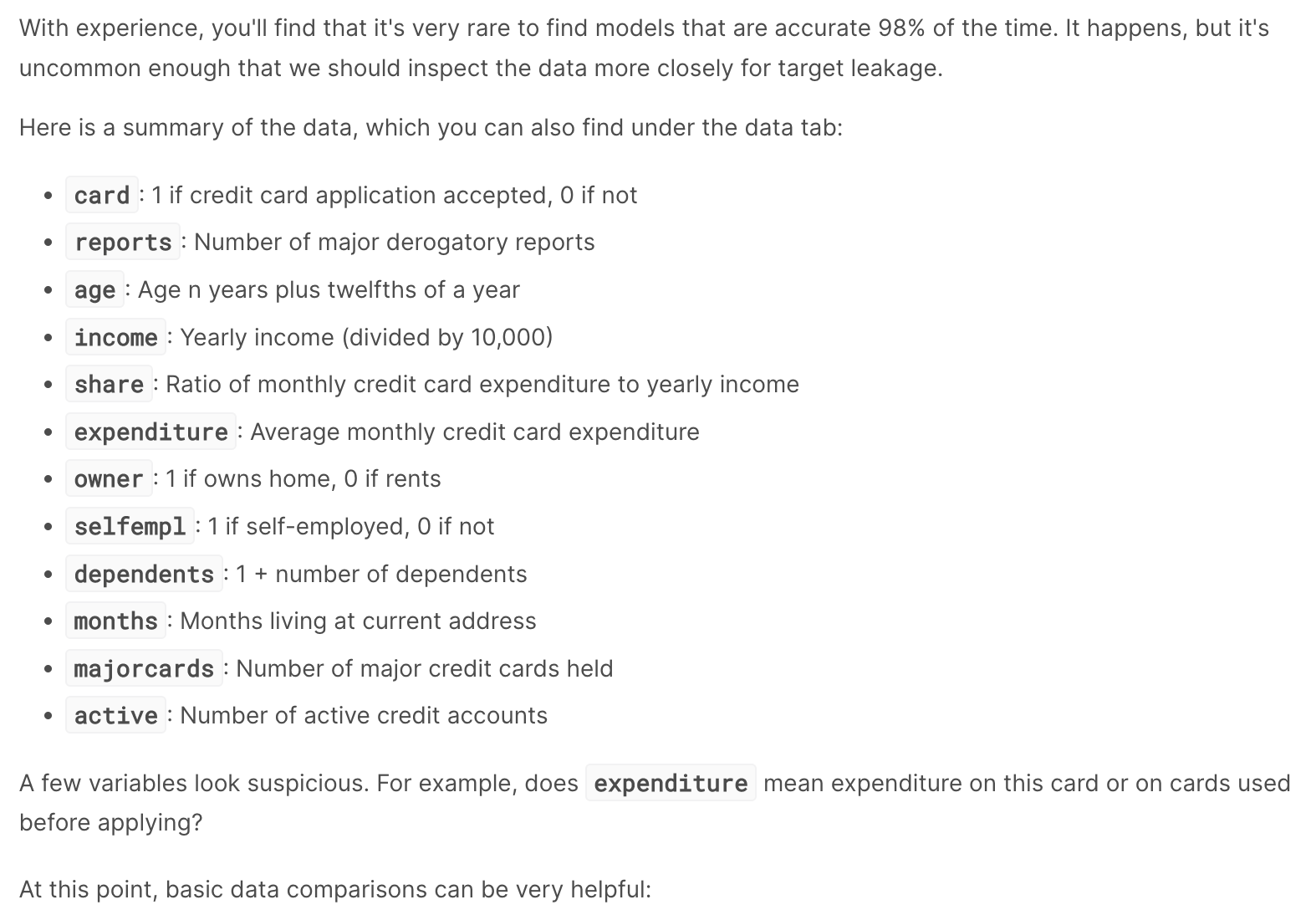
data = pd.read_csv('../input/aer-credit-card-data/AER_credit_card_data.csv',
true_values = ['yes'], false_values = ['no'])

y = data.card
X = data.drop(['card'], axis=1)

print("Number of rows in the dataset:", X.shape[0]) # Number of rows in the dataset: 1319
X.head()
reports age income share expenditure owner selfemp dependents months majorcards active
0 0 37.66667 4.5200 0.033270 124.983300 True False 3 54 1 12
1 0 33.25000 2.4200 0.005217 9.854167 False False 3 34 1 13
2 0 33.66667 4.5000 0.004156 15.000000 True False 4 58 1 5
3 0 30.50000 2.5400 0.065214 137.869200 False False 0 25 1 7
4 0 32.16667 9.7867 0.067051 546.503300 True False 2 64 1 5
from sklearn.pipeline import make_pipeline
from sklearn.ensemble import RandomForestClassifier
from sklearn.model_selection import cross_val_score

# Since there is no preprocessing, we don't need a pipeline (used anyway as best practice!)
my_pipeline = make_pipeline(RandomForestClassifier(n_estimators=100))
cv_scores = cross_val_score(my_pipeline, X, y,
cv=5,
scoring='accuracy')

print("Cross-validation accuracy: %f" % cv_scores.mean())
# Cross-validation accuracy: 0.981052

image-20230423181238348

expenditures_cardholders = X.expenditure[y]
expenditures_noncardholders = X.expenditure[~y]

print('Fraction of those who did not receive a card and had no expenditures: %.2f' \
%((expenditures_noncardholders == 0).mean()))
print('Fraction of those who received a card and had no expenditures: %.2f' \
%(( expenditures_cardholders == 0).mean()))

# Fraction of those who did not receive a card and had no expenditures: 1.00
# Fraction of those who received a card and had no expenditures: 0.02

image-20230423181719683

# Drop leaky predictors from dataset
potential_leaks = ['expenditure', 'share', 'active', 'majorcards']
X2 = X.drop(potential_leaks, axis=1)

# Evaluate the model with leaky predictors removed
cv_scores = cross_val_score(my_pipeline, X2, y,
cv=5,
scoring='accuracy')

print("Cross-val accuracy: %f" % cv_scores.mean())
train-test contamination

训练-测试数据污染指的是,在模型评估时,使用了测试集中的信息来进行训练。这可能会导致模型在测试集上表现良好,但在实际应用中却无法取得同样的效果。例如,如果在特征缩放时使用了整个数据集的信息,包括测试集,那么测试集的信息就会泄漏到训练集中,导致模型在测试集上表现得过于优秀。

Time Series

Linear Regression With Time Series

Use two features unique to time series: lags and time steps.

import pandas as pd

df = pd.read_csv(
"../input/ts-course-data/book_sales.csv",
index_col='Date',
parse_dates=['Date'],
).drop('Paperback', axis=1)

df.head()
Hardcover
Date
2000-04-01 139
2000-04-02 128
2000-04-03 172
2000-04-04 139
2000-04-05 191

线性回归算法学习如何从其输入特征中进行加权和。对于两个特征,我们将拥有:

target = weight_1 * feature_1 + weight_2 * feature_2 + bias
Time-step features
import numpy as np
df['Time'] = np.arange(len(df.index))
df.head()
Hardcover Time
Date
2000-04-01 139 0
2000-04-02 128 1
2000-04-03 172 2
2000-04-04 139 3
2000-04-05 191 4

线性回归加入时间虚拟变量的模型结果为:

target = weight * time + bias

The time dummy then lets us fit curves to time series in a time plot, where Time forms the x-axis.

image-20230423200240833

Lag features
df['Lag_1'] = df['Hardcover'].shift(1)
df = df.reindex(columns=['Hardcover', 'Lag_1'])

df.head()
Hardcover Lag_1
Date
2000-04-01 139 NaN
2000-04-02 128 139.0
2000-04-03 172 128.0
2000-04-04 139 172.0
2000-04-05 191 139.0

带滞后特征的线性回归得到模型:

target = weight * lag + bias

滞后特征(lag features)可以让我们对滞后图(lag plots)进行曲线拟合,其中系列中的每个观测值都与前一个观测值绘制在图中。image-20230423200922759

Example - Tunnel Traffic